Quantifying Variability: Variance, Standard Deviation, and Coefficient of Variation

When we have the whole population, each data point is known so you are 100% sure of the measures we are calculating.

When we take a sample of this population and compute a sample statistic, it is interpreted as an approximation of the population parameter.

Moreover, if we extract 10 different samples from the same population, we will get 10 different measures.

Statisticians have solved the problem by adjusting the algebraic formulas for many statistics to reflect this issue. Therefore, we will explore both population and sample formulas, as they are both used.

You must be asking yourself why there are unique formulas for the mean, median and mode. Well, actually, the sample mean is the average of the sample data points, while the population mean is the average of the population data points. As you can see in the picture below, there are two different formulas, but technically, they are computed in the same way.

After this short clarification, it’s time to get onto variance.

Variance measures the dispersion of a set of data points around their mean value.

Population variance, denoted by sigma squared, is equal to the sum of squared differences between the observed values and the population mean, divided by the total number of observations.

Sample variance, on the other hand, is denoted by s squared and is equal to the sum of squared differences between observed sample values and the sample mean, divided by the number of sample observations minus 1.

When you are getting acquainted with statistics, it is hard to grasp everything right away. Therefore, let’s stop for a second to examine the formula for the population and try to clarify its meaning. The main part of the formula is its numerator, so that’s what we want to comprehend.

The sum of differences between the observations and the mean, squared. So, this means that the closer a number is to the mean, the lower the result we obtain will be. And the further away from the mean it lies, the larger this difference.

Squaring the differences has two main purposes.

First, by squaring the numbers, we always get non-negative computations. Without going too deep into the mathematics of it, it is intuitive that dispersion cannot be negative. Dispersion is about distance and distance cannot be negative.

If, on the other hand, we calculate the difference and do not elevate to the second degree, we would obtain both positive and negative values that, when summed, would cancel out, leaving us with no information about the dispersion.

Second, squaring amplifies the effect of large differences. For example, if the mean is 0 and you have an observation of 100, the squared spread is 10,000!

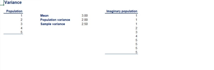
Alright, enough dry theory. It is time for a practical example. We have a population of five observations – 1, 2, 3, 4 and 5. Let’s find its variance.

We start by calculating the mean: (1 + 2 + 3 + 4 + 5) / 5 = 3.

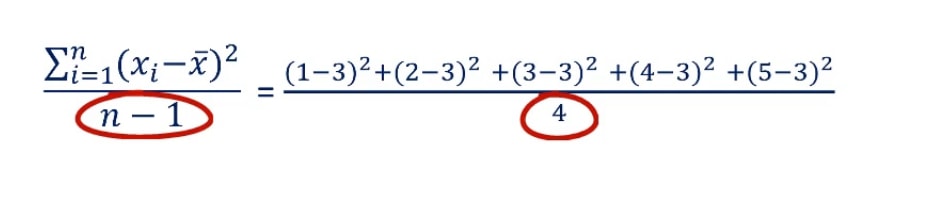
Then we apply the formula which we just discussed:

((1 – 3)2 + (2 – 3)2+ (3 – 3)2 + (4 – 3)2 + (5 – 3)2) / 5.

When we do the math, we get 2. So, the population variance of the data set is 2.

But what about the sample variance? This would only be suitable if we were told that these five observations were a sample drawn from a population. So, let’s imagine that’s the case. The sample mean is once again 3. The numerator is the same, but the denominator is going to be 4, instead of 5.

This gives us a sample variance of 2.5.

To conclude the variance topic, we should interpret the result. Why is the sample variance bigger than the population variance? In the first case, we knew the population. That is, we had all the data and we calculated the variance. In the second case, we were told that 1, 2, 3, 4 and 5 was a sample, drawn from a bigger population.

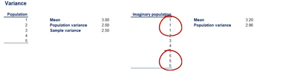
Imagine that the population of the sample were the following 9 numbers: 1, 1, 1, 2, 3, 4, 5, 5 and 5.

Clearly, the numbers are the same, but there is a concentration around the two extremes of the data set – 1 and 5. The variance of this population is 2.96.

So, our sample variance has rightfully corrected upwards in order to reflect the higher potential variability. This is the reason why there are different formulas for sample and population data.

While variance is a common measure of data dispersion, in most cases the figure you will obtain is pretty large. Moreover, it is hard to compare because the unit of measurement is squared. The easy fix is to calculate its square root and obtain a statistic known as standard deviation.

In most analyses, standard deviation is much more meaningful than variance.

Similar to the variance there is also population and sample standard deviation. The formulas are: the square root of the population variance and square root of the sample variance respectively. I believe there is no need for an example of the calculation. Anyone with a calculator in their hands will be able to do the job.

The last measure which we will introduce is the coefficient of variation. It is equal to the standard deviation, divided by the mean.

Another name for the term is relative standard deviation. This is an easy way to remember its formula – it is simply the standard deviation relative to the mean.

As you probably guessed, there is a population and sample formula once again.

So, standard deviation is the most common measure of variability for a single data set. But why do we need yet another measure such as the coefficient of variation? Well, comparing the standard deviations of two different data sets is meaningless, but comparing coefficients of variation is not.

Aristotle once said:

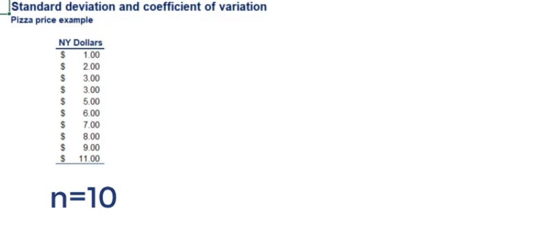
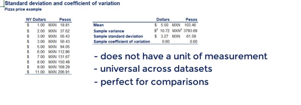
To make sure you remember, here’s an example of a comparison between standard deviations. Let’s take the prices of pizza at 10 different places in New York. As you can see in the picture below, they range from 1 to 11 dollars.

Now, imagine that you only have Mexican pesos. To you, the prices will look more like 18.81 pesos to 206.91 pesos, given the exchange rate of 18.81 pesos for one dollar.

Let’s combine our knowledge so far and find the standard deviations and coefficients of variation of these two data sets.

Sample or Population DataFirst, we have to see if this is a sample or a population. Are there only 11 restaurants in New York? Of course not. This is obviously a sample drawn from all the restaurants in the city. Then we have to use the formulas for sample measures of variability.Finding the MeanSecond, we have to find the mean. The mean in dollars is equal to 5.5 and the mean in pesos to 103.46.Calculating the Sample Variance and the Standard DeviationThe third step of the process is finding the sample variance. Following the formula that we went over earlier, we can obtain 10.72 dollars squared and 3793.69 pesos squared.The respective sample standard deviations are 3.27 dollars and 61.59 pesos, as shown in the picture below.A Few Observations

Let’s make a couple of observations.

First, variance gives results in squared units, while standard deviation in original units, as shown below.

This is the main reason why professionals prefer to use standard deviation as the main measure of variability. It is directly interpretable. Squared dollars mean nothing, even in the field of statistics.

Second, we got standard deviations of 3.27 and 61.59 for the same pizza at the same 11 restaurants in New York City. However, this seems wrong. Let’s make it right by using our last tool – the coefficient of variation.

We can divide the standard deviations by the respective means. As you can see in the picture below, we get the two coefficients of variation.

The result is the same – 0.60.

Important: Notice that it is not dollars, pesos, dollars squared or pesos squared. It is just 0.60.

This shows us the great advantage that the coefficient of variation gives us. Now, we can confidently say that the two data sets have the same variability, which was what we expected beforehand.

In the picture above, you can see the main advantages of the coefficient of variation.

To recap, there are three main measures of variability – variance, standard deviation and coefficient of variation. Each of them has different strengths and applications. Usually, we prefer standard deviation over variance because it is directly interpretable. However, the coefficient of variation has its edge over standard deviation when it comes to comparing data. After reading this tutorial, you should feel confident using all of them.

Now, using measures when working with one variable probably seems like a piece of cake. However, what if there were 2 variables? Will you be able to represent their relationship? If your answer is no, feel free to jump onto our next tutorial, in order to turn that no into a yes.

Or, if you’re considering a career in data science, check out our articles: The Data Scientist Profile, The 5 Skills You Need to Match Any Data Science Job Description, 10 Pro Tips to Make Your Resume One of a Kind, and 15 Data Science Consulting Companies Hiring Now.

***

Check out the complete Data Science Program today. We also offer a free preview version of the Data Science Program. You’ll receive 12 hours of beginner to advanced content for free. It’s a great way to see if the program is right for you.